ERP analysis of UCAP data

Loading R packages

library("reticulate")
library("Rmisc")
library("dplyr")
library("ggplot2")
library("lme4")

Loading the pipeline

After following the installation instructions for R users, we can use the reticulate Package to load the Python pipeline package directly from R.

pipeline <- import("pipeline")

Downloading example data

The pipeline comes with a function to download example data from the Abdel Rahman Lab’s UCAP study. In this EEG experiment, participants performed a visual search task with visual objects that were either presented visually intact (factor n_b == "normal") or blurred (factor n_b == "blurr").

The raw data are stored in the Open Science Framework and more details about the study are in Frömer et al. (2018).

ucap_files <- pipeline$datasets$get_ucap(participants = 2)
print(ucap_files)

$raw_files
[1] "/home/docs/.cache/hu-neuro-pipeline/ucap/raw/05.vhdr"
[2] "/home/docs/.cache/hu-neuro-pipeline/ucap/raw/07.vhdr"

$besa_files
[1] "/home/docs/.cache/hu-neuro-pipeline/ucap/cali/05_cali.matrix"
[2] "/home/docs/.cache/hu-neuro-pipeline/ucap/cali/07_cali.matrix"

$log_files
[1] "/home/docs/.cache/hu-neuro-pipeline/ucap/log/5_test.txt"
[2] "/home/docs/.cache/hu-neuro-pipeline/ucap/log/7_test.txt"

To save time, we only download and process data from the first two participants. Feel free to re-run the example with more participants by increasing or removing the n_participants argument.

The paths of the downloaded EEG header files (.vhdr), behavioral log files (.txt), and ocular correction files (.matrix) can now be fed into pipeline.

Running the pipeline

We run a simple pipeline for single-trial ERP analysis with the following steps:

• Downsampling to 250 Hz

• Re-referencing to common average (per default)

• Ocular correction with BESA/MSEC matrices

• Default bandpass filtering between 0.1 and 40 Hz (per default)

• Segmentation to epochs around stimulus triggers

• Baseline correction (per default)

• Rejecting bad epochs based on peak-to-peak amplitudes > 200 µV (per default)

• Computing single trial N2 and P3b amplitudes by averaging across time windows and channels of interest

• Creating by-participant averages for the blurred and normal conditions

res <- pipeline$group_pipeline(

  # Input/output paths
  raw_files = ucap_files$raw_files,
  log_files = ucap_files$log_files,
  output_dir = "output",

  # Preprocessing options
  downsample_sfreq = 250.0,
  besa_files = ucap_files$besa_files,

  # Epoching options
  triggers = c(201:208, 211:218),
  components = list(
    "name" = list("N2", "P3b"),
    "tmin" = list(0.25, 0.4),
    "tmax" = list(0.35, 0.55),
    "roi" = list(
      c("FC1", "FC2", "C1", "C2", "Cz"),
      c("CP3", "CP1", "CPz", "CP2", "CP4", "P3", "Pz", "P4", "PO3", "POz", "PO4")
    )
  ),

  # Averaging options
  average_by = list(
    blurr = "n_b == 'blurr'",
    normal = "n_b == 'normal'"
  )
)

See the Input arguments page for a list of all available processing options.

Checking the results

The resulting object (res) is a list with three components: A dataframe of single trial ERP amplitudes, a dataframe of by-participant condition averages, and a dictionary of pipeline metadata.

str(res, max.level = 1)

List of 3
 $ :'data.frame':	3840 obs. of  32 variables:
  ..- attr(*, "pandas.index")=RangeIndex(start=0, stop=3840, step=1)
 $ :'data.frame':	2000 obs. of  69 variables:
  ..- attr(*, "pandas.index")=RangeIndex(start=0, stop=2000, step=1)
 $ :List of 45

Single-trial ERP amplitudes

These are basically just the log files, concatenated for all participants, with two added columns for the two ERP components of interest. Each value in these columns reflects the single trial ERP amplitude, averaged across time points and channels of interest.

Here are the first couple of lines of the dataframe:

trials <- res[[1]]
head(trials)

A data.frame: 6 × 32

	participant_id	VPNummer	version	wdh	lfdNr	n_b	Standard	Deviant	Objektpaar	BedCode_alt	⋯	Pos5	Pos6	Pos7	Pos8	Pos9	Pos10	Pos11	Pos12	N2	P3b
	<chr>	<dbl>	<dbl>	<dbl>	<dbl>	<chr>	<chr>	<chr>	<dbl>	<chr>	⋯	<chr>	<chr>	<chr>	<chr>	<chr>	<chr>	<chr>	<chr>	<dbl>	<dbl>
1	05	5	1	1	1	normal	objekt7.bmp	objekt8.bmp	8	gngf	⋯	objekt7.bmp	objekt7.bmp	objekt7.bmp	objekt7.bmp	objekt7.bmp	objekt7.bmp	objekt7.bmp	objekt7.bmp	-0.3113551	-9.026910
2	05	5	1	1	2	blurr	objekt3blurr7.bmp	objekt1blurr7.bmp	10	un	⋯	objekt3blurr7.bmp	objekt3blurr7.bmp	objekt3blurr7.bmp	objekt3blurr7.bmp	objekt3blurr7.bmp	objekt3blurr7.bmp	objekt3blurr7.bmp	objekt1blurr7.bmp	-9.7551663	-8.773690
3	05	5	1	1	3	blurr	objekt3blurr7.bmp	objekt1blurr7.bmp	10	un	⋯	objekt3blurr7.bmp	objekt3blurr7.bmp	objekt1blurr7.bmp	objekt3blurr7.bmp	objekt3blurr7.bmp	objekt3blurr7.bmp	objekt3blurr7.bmp	objekt3blurr7.bmp	0.1606203	2.467171
4	05	5	1	1	4	normal	objekt2.bmp	objekt4.bmp	3	un	⋯	objekt2.bmp	objekt2.bmp	objekt2.bmp	objekt2.bmp	objekt2.bmp	objekt2.bmp	objekt2.bmp	objekt2.bmp	0.1463861	-4.720746
5	05	5	1	1	5	normal	objekt8.bmp	objekt6.bmp	15	unuf	⋯	objekt8.bmp	objekt8.bmp	objekt8.bmp	objekt8.bmp	objekt8.bmp	objekt8.bmp	objekt8.bmp	objekt6.bmp	4.2821534	1.850902
6	05	5	1	1	6	normal	objekt6.bmp	objekt8.bmp	7	unuf	⋯	objekt6.bmp	objekt6.bmp	objekt6.bmp	objekt6.bmp	objekt6.bmp	objekt6.bmp	objekt6.bmp	objekt6.bmp	-3.7349591	-4.243824

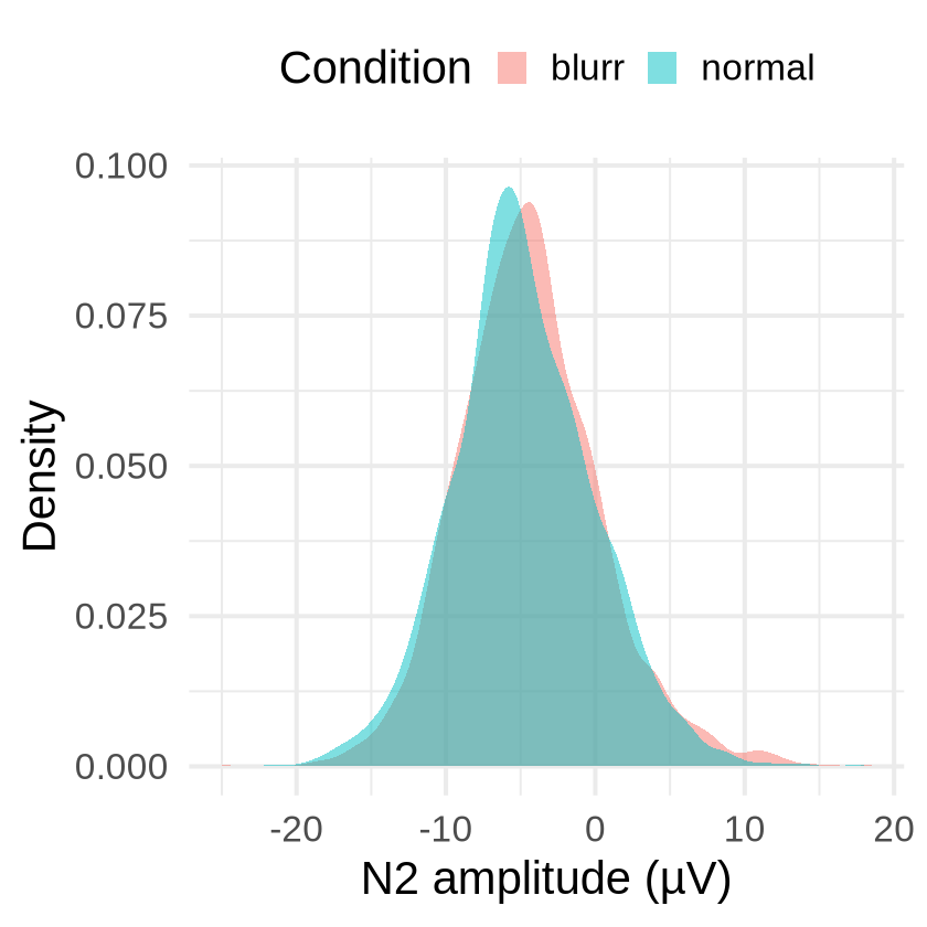
We can plot the single trial ERP amplitudes (here for the N2 component), separately for the blurred and normal conditions, e.g., as a density plot:

trials |>
  ggplot(aes(x = N2, fill = n_b)) +
  geom_density(color = NA, alpha = 0.5) +
  labs(x = "N2 amplitude (µV)", y = "Density", fill = "Condition") +
  theme_minimal(base_size = 25.0) +
  theme(legend.position = "top")

Warning message:
“Removed 5 rows containing non-finite outside the scale range
(`stat_density()`).”

Raincloud plots (Allen et al., 2021) would be a fancier alternative (e.g., using the ggrain package).

Note that these kinds of plots do not take into account the fact that the single trial amplitudes are nested within participants (and/or items). To do this, and to quantify if any descriptive differences between conditions are statistically reliable, we can run a linear mixed-effects model:

mod <- lmer(N2 ~ n_b + (1 | participant_id), data = trials)
summary(mod)

Linear mixed model fit by REML ['lmerMod']
Formula: N2 ~ n_b + (1 | participant_id)
   Data: trials

REML criterion at convergence: 22662.2

Scaled residuals: 
    Min      1Q  Median      3Q     Max 
-4.6840 -0.6285  0.0027  0.6094  5.1771 

Random effects:
 Groups         Name        Variance Std.Dev.
 participant_id (Intercept)  2.521   1.588   
 Residual                   21.524   4.639   
Number of obs: 3835, groups:  participant_id, 2

Fixed effects:
            Estimate Std. Error t value
(Intercept)  -4.4039     1.1276  -3.906
n_bnormal    -0.3920     0.1498  -2.616

Correlation of Fixed Effects:
          (Intr)
n_bnormal -0.066

Here we predict the single trial N2 amplitude based on the fixed effect of blurred vs. normal, and we allow for random variation in the intercept between participants.

Note that for sound inference on the full dataset, we would want to:

• apply proper contrast coding to the n_b factor (e.g., Schad et al., 2020),

• include random effects not just for participants, but also for items (e.g., Judd et al., 2012), and

• include not just random intercepts, but also random slopes (e.g., Barr et al., 2013).

By-participant condition averages

This is one big data frame which, unlike trials, is averaged across trials (i.e., losing any single trial information) but not averaged across time points or channels (i.e., retaining the millisecond-wise ERP waveform at all electrodes).

evokeds <- res[[2]]
head(evokeds)

A data.frame: 6 × 69

	participant_id	label	query	time	Fp1	Fpz	Fp2	AF7	AF3	AFz	⋯	POz	PO4	PO8	PO10	O1	Oz	O2	A2	N2	P3b
	<chr>	<chr>	<chr>	<dbl>	<dbl>	<dbl>	<dbl>	<dbl>	<dbl>	<dbl>	⋯	<dbl>	<dbl>	<dbl>	<dbl>	<dbl>	<dbl>	<dbl>	<dbl>	<dbl>	<dbl>
1	05	blurr	n_b == 'blurr'	-0.500	-0.4606889	-1.177251	-1.329169	-0.6407359	-1.0136561	-1.663345	⋯	1.326010	0.4672807	-0.5412924	-0.08421176	0.6745672	0.9986516	0.4336516	17.40658	-0.05420106	1.204583
2	05	blurr	n_b == 'blurr'	-0.496	-0.3794556	-1.124926	-1.167457	-0.6382813	-0.7834862	-1.487443	⋯	1.294548	0.3869416	-0.6668954	-0.17910905	0.6571419	0.9351367	0.3286029	17.43751	-0.06377263	1.152653
3	05	blurr	n_b == 'blurr'	-0.492	-0.3059947	-1.130408	-1.096503	-0.6251941	-0.8076923	-1.338292	⋯	1.313320	0.4182054	-0.6730624	-0.22483241	0.6443670	0.9016988	0.2835874	17.37792	-0.04986672	1.138065
4	05	blurr	n_b == 'blurr'	-0.488	-0.2548575	-1.172944	-1.123665	-0.5749940	-0.9672618	-1.293291	⋯	1.361784	0.5391044	-0.5782835	-0.23259965	0.6162911	0.8827936	0.2931589	17.72110	-0.03514376	1.151694
5	05	blurr	n_b == 'blurr'	-0.484	-0.2465241	-1.217320	-1.192534	-0.5028769	-1.0955399	-1.371385	⋯	1.413782	0.7041170	-0.4335859	-0.22822905	0.5573336	0.8582450	0.3340357	17.56499	-0.04762919	1.174367
6	05	blurr	n_b == 'blurr'	-0.480	-0.2809327	-1.234611	-1.239649	-0.4534182	-1.1279311	-1.513666	⋯	1.453795	0.8739736	-0.2852284	-0.22749856	0.4733733	0.8252039	0.3843244	17.61845	-0.09389271	1.191099

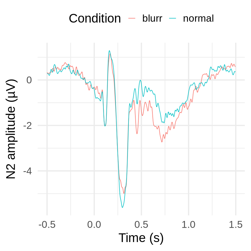
We can use it to display the grand-averaged ERP waveforms for different conditions as a timecourse plot at a single channel or ROI (here for the N2 ROI):

evokeds |>
  ggplot(aes(x = time, y = N2, color = label)) +
  stat_summary(geom = "line", fun = mean) +
  labs(x = "Time (s)", y = "N2 amplitude (µV)", color = "Condition") +
  theme_minimal(base_size = 25.0) +
  theme(legend.position = "top")

We can add error bars to the waveforms using the appropriate standard error for whin-participant variables:

evokeds |>
  summarySEwithin(
    measurevar = "N2",
    withinvars = c("label", "time"),
    idvar = "participant_id"
  ) |>
  mutate(time = as.numeric(as.character(time))) |>
  ggplot(aes(x = time, y = N2)) +
  geom_ribbon(aes(ymin = N2 - se, ymax = N2 + se, fill = label), alpha = 0.2) +
  geom_line(aes(color = label)) +
  labs(
    x = "Time (s)",
    y = "N2 amplitude (µV)",
    color = "Condition",
    fill = "Condition"
  ) +
  theme_minimal(base_size = 25.0) +
  theme(legend.position = "top")

Automatically converting the following non-factors to factors: label, time

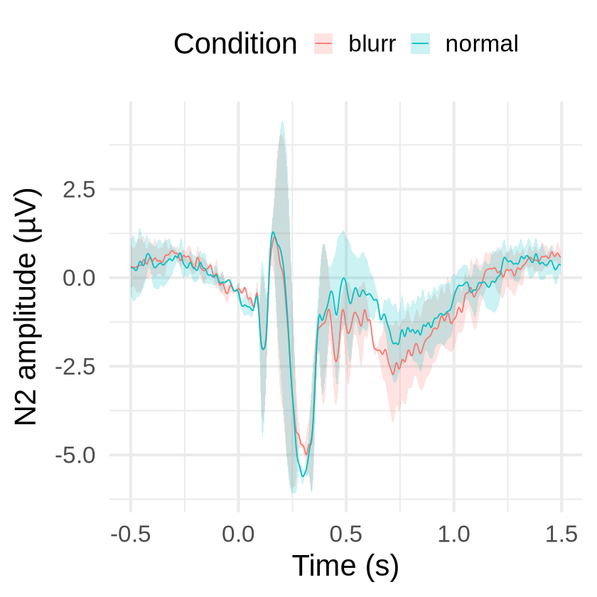
Note that (a) these error bars do not necessarily have to agree with the mixed model inference above, since one is performed on data averaged across trials and the other on data averaged across time, and (b) that the error bars in this example are very large and noisy because they are based on only two participants.

Pipeline metadata

This is a dictionary (i.e., a named list) with various metadata about the pipeline run.

config <- res[[3]]
names(config)

1. 'raw_files'
2. 'log_files'
3. 'output_dir'
4. 'clean_dir'
5. 'epochs_dir'
6. 'report_dir'
7. 'to_df'
8. 'downsample_sfreq'
9. 'veog_channels'
10. 'heog_channels'
11. 'montage'
12. 'bad_channels'
13. 'ref_channels'
14. 'besa_files'
15. 'ica_method'
16. 'ica_n_components'
17. 'highpass_freq'
18. 'lowpass_freq'
19. 'triggers'
20. 'triggers_column'
21. 'epochs_tmin'
22. 'epochs_tmax'
23. 'baseline'
24. 'skip_log_rows'
25. 'skip_log_conditions'
26. 'reject_peak_to_peak'
27. 'components'
28. 'average_by'
29. 'perform_tfr'
30. 'tfr_subtract_evoked'
31. 'tfr_freqs'
32. 'tfr_cycles'
33. 'tfr_mode'
34. 'tfr_baseline'
35. 'tfr_components'
36. 'perm_contrasts'
37. 'perm_tmin'
38. 'perm_tmax'
39. 'perm_channels'
40. 'perm_fmin'
41. 'perm_fmax'
42. 'n_jobs'
43. 'vhdr_files'
44. 'auto_rejected_epochs'
45. 'package_versions'

It includes any input arguments that were used by the pipeline (either user-specified or default values). Additionally, it contains some statistics that were automatically computed by the pipeline along the way, such as the number of rejected epochs (based on a peak-to-peak amplitude threshold) per participant:

lengths(config$auto_rejected_epochs)

05

5

07

0

Finally, it records the Python version and the versions of the most important Python packages that were used by the pipeline:

config$package_versions

$python

'3.11.8'

$pipeline

'0.8.6.dev0'

$mne

'1.6.1'

$numpy

'1.26.4'

$pandas

'2.2.2'

$`scikit-learn`

'1.4.2'